Introduction

What is Machine Learning?

two definitions of Machine Learning

1. Arthur Samuel described it as: "the field of study that gives computers the ability to learn without being explicitly programmed." This is an older, informal definition.

2. Tom Mitchell provides a more modern definition: "A computer program is said to learn from experience E with respect to some class of tasks T and performance measure P, if its performance at tasks in T, as measured by P, improves with experience E."

   • Example: playing checkers.

     E = the experience of playing many games of checkers

     T = the task of playing checkers.

     P = the probability that the program will win the next game.

any machine learning problem can be assigned to one of two broad classifications

1. supervised learning
2. unsupervised learning

Supervised Learning

In supervised learning, we are given a data set and already know what our correct output should look like, having the idea that there is a relationship between the input and the output.

supervised learning problems are categorized into

1. regression
   • predict results within a continuous output, meaning that mapping input variables to some continuous function
   • examples
     • predict housing price
     • predict person's age on the basis of the given picture
2. classification
   • predict results in a discrete output , meaning that mapping input variables into discrete categories
   • example
     • predict whether the tumor is malignant or benign

Unsupervised Learning

Unsupervised learning allows us to approach problems with little or no idea what our results should look like. We can derive structure from data where we don't necessarily know the effect of the variables.

We can derive this structure by clustering the data based on relationships among the variables in the data.

With unsupervised learning there is no feedback based on the prediction results.

Example:

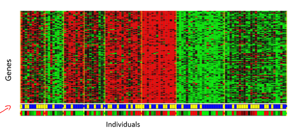
1. Clustering: Take a collection of 1,000,000 different genes, and find a way to automatically group these genes into groups that are somehow similar or related by different variables, such as lifespan, location, roles, and so on.

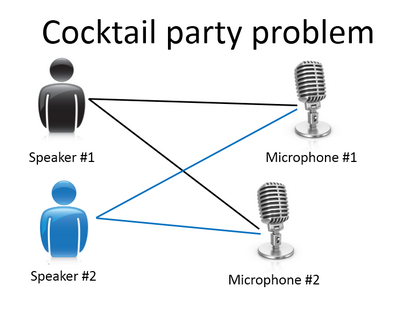
2. Non-clustering: The "Cocktail Party Algorithm", allows you to find structure in a chaotic environment. (i.e. identifying individual voices and music from a mesh of sounds at a cocktail party).

Linear Regression with One Variable

Model Representation

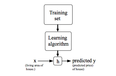
$$ \begin{array}{l}{\text { To establish notation for future use } x^{(i)} \text { to denote the "input" variables (living area in this example) also called input }} \\ {\text { features, and } y^{(i)} \text { to denote the "output" or target variable that we are tring t(price). A pair }\left(x^{i}\right), y^{(i)} \text { is called a }} \\ {\text { training example, and the dataset that well be learn-alist of mtraining examples }\left(x^{(i)}, y^{(i)}\right) ; i=1, \ldots, m \text { -is called }}{\text { atraining set. }} \\{ \text {Note that the superscript tip the notation is simply an index into the training set, and has nothing to dowith }} \\ {\text { exponentiaxtion. We will also use } x \text { to denote the space of input values, and } Y \text { to denote the space of output vautput values. In this }} \\ {\text { example, } x=Y=R .}\end{array} $$

To describe the supervised learning problem slightly more formally, our goal is, given a training set, to learn a function h : X → Y so that h(x) is a “good” predictor for the corresponding value of y. For historical reasons, this function h is called a hypothesis. Seen pictorially, the process is therefore like this:

When the target variable that we’re trying to predict is continuous, such as in our housing example, we call the learning problem a regression problem. When y can take on only a small number of discrete values (such as if, given the living area, we wanted to predict if a dwelling is a house or an apartment, say), we call it a classification problem.

Cost Function

损失函数(Loss/Error Function): 计算单个样本的误差。
代价函数(Cost Function): 计算整个训练集所有损失函数之和的平均值。

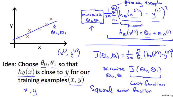
We can measure the accuracy of our hypothesis function by using a cost function. This takes an average difference (actually a fancier version of an average) of all the results of the hypothesis with inputs from x's and the actual output y's. $$ J\left(\theta_{0}, \theta_{1}\right)=\frac{1}{2 m} \sum_{i=1}^{m}\left(\hat{y}_{i}-y_{i}\right)^{2}=\frac{1}{2 m} \sum_{i=1}^{m}\left(h_{\theta}\left(x_{i}\right)-y_{i}\right)^{2} $$

$$ \begin{array}{l}{\text { To break it apart, it is } \frac{1}{2} \bar{x} \text { where } \bar{x} \text { is the mean of the squares of } h_{\theta}\left(x_{i}\right)-y_{i} \text { or the difference between the predicted value and }} \\ {\text { the actual value. }} \\ {\text { This function is otherwise called the "squared error function", or "N-Nean square". The mean is halved }\left(\frac{1}{2}\right) \text { as a }} \\ {\text { convention is otherwise called the gradied erroctiont, as the derivative term of the square function will cancel out the } \frac{1}{2}} \\ {\text { torm. The following image summarizes what the cost function does: }}\end{array} $$